More Examples¶

This chapter shows several common examples to illusrate how the model specification DSL works in practice.

Latent Dirichlet Allocation¶

Latent Dirichlet Allocation (LDA) is a probabilistic model for topic modeling. The basic idea is to use a set of topics to describe documents. Key aspects of this model is summarized below:

Each document is considered as a bag of words, which means that only the frequencies of words matter, while the sequential order is ignored. In practice, each document is summarized by a histogram vector $h$ .
The model comprises a set of topics. We denote the number of topics by $K$ . Each topic is characterized by a distribution over vocabulary, denoted by $\beta_k$ . It is a common practice to place a Dirichlet prior over these distributions.
Each document is associated with a topic proportion vector $\theta$ , generated from a Dirichlet prior.
Each word in a document is generated independently. Specifically, a word is generated as follows

$z_i &\ \sim \ \theta \\ w_i | z_i &\ \sim \ \beta_{z_i}$

Here, $z_i$ indicates the topic associated with the word $w_i$ .

The model specification is then given by

@model LatentDirichletAllocation begin
    # constants
    @constant m::Int      # vocabulary size
    @constant n::Int      # number of documents
    @constant nw::Vector{Int}    # numbers of words in documents

    @hyperparam K::Int      # number of topics
    @hyperparam a::Float64  # Dirichlet hyper-prior for beta

    # parameters
    @param alpha :: (0.0 .. Inf)^K
    for k in 1 : K
        @param beta[k] ~ Dirichlet(a)
    end

    # documents
    for i in 1 : n
        theta[i] ~ Dirichlet(alpha)
        let p = sum(beta[k] * theta[i][k] for k in 1 : K)
            h[i] ~ Multinomial(nw[i], p)
        end
    end
end

Here, the keyword let introduces a local value p to denote the sum vector. It is important to note that p has a local scope (thus it is not visible outside the loop), and the value of p can be different for different i.

The following function learns an LDA model from word histograms of training documents.

function learn_lda(h::Matrix{Double}, K::Int, alpha::Float64)
    learn_model(LatentDirichletAllocation(
        m = size(h, 1), n = size(h, 2), nw = sum(h, 1), K = K, a = alpha),
        {:h => columns(h)})
end

mdl = learn_lda(training_hists, K, alpha)

The following statement infers topic proportions of testing documents, given a learned LDA model.

# suppose mdl is a learned LDA model
theta = query(mdl, {:h => columns(testing_corpus)}, :theta)

Hidden Markov Model¶

Hidden Markov Model (HMM) is a popular model to describe dynamic processes. It assumes that the observed process is driven by a latent Markov chain, and the observation at each time step is independently generated conditioned on the latent states at the same time. A time-homogeneous Markov model is characterized by an initial distribution of states, denoted by $\pi$ , a transition probability matrix, denoted by $T$ , and an observation model that generates observations based on latent states. 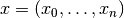Each sample of a Hidden Markov model is a sequence $x = (x_0, \ldots, x_n)$ , where the observation $x_t$ is associated with a latent state $s_t$ . The joint distribution over both the observations and the states is given by

$p(x, s) = \pi(x_0) \prod_{t=1}^n T(x_{t-1}, x_t) \prod_{t=0}^n p(x_t | s_t; \theta).$

Here, $\theta$ denotes the parameter of the observation model.

Generally, the component models associated with the observations can be any distributions. Therefore, HMM is actually a family of distributions that can be specified using a generic specification, as below:

@model HiddenMarkovModel{G, ParamTypes} begin
    @constant n::Int    # number of sequences
    @constant len::Vector{Int}   # the sequence lengths
    @hyperparam K::Int    # the size of latent state space

    # parameters
    @param pi :: (0.0 .. 1.0)^K        # initial distribution
    @param T :: (0.0 .. 1.0)^(K, K)    # transition probability matrix

    for k in 1 : K
        for j in 1 : length(ParamTypes)
            @param theta[k][j] :: ParamTypes[j]
        end
    end

    # sequences
    for i in 1 : n
        z[i][1] ~ Categorical(pi)
        for t = 2 : len[i]
            z[i][t] ~ Categorical(T[z[t-1], :])
        end

        for t in 1 : len[i]
            let s = z[i][t]
                x[i][t] ~ G(theta[s]...)
            end
        end
    end
end

To construct an HMM with K Gaussian components, one can write:

@modelalias HiddenMarkovGaussModel HiddenMarkovModel{G, Params} begin
    @constant d::Int    # vector space dimension
    @with G = MultivariateNormal
    @with Params[1] = Float64^d
    @with Params[2] = Float64^(d, d)
end

The following query function learns a HMM (with Gaussian components):

function learn_hmm(seqs, K::Int)
    # seqs is a collection of observed sequences
    # K is the number of latent states

    learn_model(HiddenMarkovGaussModel(
        n = length(seqs), len = map(length, seqs), K = K),
        {:x => seqs})
end

mdl = learn_hmm(seqs, K)

The following query draws samples of the latent state sequences, given a learned HMM model and a sequences of observations.

function hmm_sample(mdl::HiddenMarkovGaussModel, obs::Matrix{Float64}, ns::Int)
    # obs is a sequence of observed features (each column for a time step)
    # ns is the number of samples to d

    query(mdl, {:x => obs}, :(sample(z, ns)))
end

# run the function to draw 100 sample state-sequendes for x
x = rand(3, 100)
y = hmm_sample(mdl, x, 100)

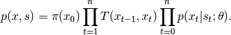
Markov Random Fields¶

Unlike Bayesian networks, which can be factorized into a product of (conditional) distributions, Markov random fields are typically formulated in terms of potentials. Generally, a MRF formulation consists of two parts: identifying relevant cliques (small subsets of directly related variables) and assigning potential functions to them. In computer vision, Markov random fields are widely used in low level vision tasks, such as image recovery and segmentation. Deep Boltzmann machines, which become increasingly popular in recent years, are actually a special form of Markov random field. Here, we use a simple MRF model in the context of image denoising to demonstrate how one can use the model specification to describe an MRF.

From a probabilistic modeling standpoint, the task of image denoising can be considered as an inference problem based on an image model combined with an observation model. An image model captures the prior knowledge as to what an clean image may look like, while the observation model describes how the observed image is generated through a noisy imaging process. Here, we consider a simple setting: Gaussian MRF prior + white noise. A classical formulation of Gaussian MRF for image modeling is given below

$p(x) = \frac{1}{Z} \exp \left( -E(x; \theta) \right).$

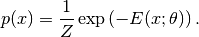
Here, the distribution is formulated in the form of a Gibbs distribution, and $E(x; \theta)$ is the energy function, which is controlled by a parameter $theta$. The energy function $E(x; theta)$ can be devised in different ways. A typical design would encourage smoothness, that is, assign low energy value when the intensity values of neighboring pixels are close to each other. For example, a classical formulation uses the following energy function

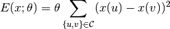
$E(x; \theta) = \theta \sum_{\{u, v\} \in \mathcal{C}} (x(u) - x(v))^2$

Here, $u$ and $v$ are indices of pixels, and the clique set $cset$ contains all edges between neighboring pixels. With the white noise assumption, the observed pixel values are given by

$y(u) = x(u) + \varepsilon(u), \quad \text{with } \varepsilon(u) \ \sim \ \mathcal{N}(0, \sigma^2).$

Below is the specification of the joint model:

@model SimpleMRF begin
    @constant nimgs::Int   # the number of images
    @constant imgsizes::Vector{(Int, Int)}

    # parameters
    @param theta::Float64     # the Gaussian MRF parameter
    @param sig::Float64       # the variance of white noise

    for t in 1 : nimgs
        let m = imgsizes[t][1], n = imgsizes[t][2]
            x[t]::Float64^(m, n)   # the true image
            y[t]::Float64^(m, n)   # the observed noisy image

            let xt = x[t], yt = y[t]
                # the image prior (Gaussian MRF)
                for i in 2 : m-1, j in 2 : n-1
                    @fac exp(-theta * (xt[i,j] - xt[i,j-1])^2)
                    @fac exp(-theta * (xt[i,j] - xt[i,j+1])^2)
                    @fac exp(-theta * (xt[i,j] - xt[i-1,j])^2)
                    @fac exp(-theta * (xt[i,j] - xt[i+1,j])^2)
                end

                # the observation model
                for i in 1 : m, j in 1 : n
                    yt[i,j] ~ Normal(xt[i,j], sig)
                end
            end
        end
    end
end

The following statement learns the model from a set of uncorrupted images

# suppose imgs is an array of images
mdl = learn_model(SimpleMRF(nimgs=length(imgs), imgsizes=map(size, imgs)), {:x=>imgs})

In this specification, four potentials are used to connect a pixel to its left, right, upper, and lower neighbors. This approach would become quite cumbersome as the neighborhood grows. Many state-of-the-art denoising algorithms use mucher larger neighborhood (e.g. 5 x 5, 9 x 9, etc) to capture high order texture structure. A representative example is the Field of Experts, where the MRF prior is defined using a set of filters as follows:

$p(x) = \frac{1}{Z} \exp \left( \sum_{k=1}^K \sum_{c \in \mathcal{C}} \rho( J_k^T x_c, \alpha_k) \right), \quad \text{with } \rho(v, \alpha) := -\alpha \log(1 + v^2).$

Here, $\mathcal{C}$ is the set of all patches of certain size (say $5 times 5$), and $x_c$ is the pixel values over a small patch $c$ . Here, $K$ filters $J_1, \ldots, J_K$ are used, and $J_k^T x_c$ is the filter response at patch $c$ . $\rho$ is a robust potential function that maps the filter responses to potential values, controlled by a parameter $\alpha$ . The specification below describes this more sophisticated model, where local functions and local variables are used to simplify the specification.

@model FieldOfExperts begin
    @constant K::Int         # the number of filters
    @constant w::Int         # patch size (w = 5 for 5 x 5 patches)
    @constant ew::Int = (w - 1) / 2  # half patch dimension
    @constant nimgs::Int     # the number of images
    @constant imgsizes::Vector{(Int, Int)}
    @constant sig :: Float64   # variance of white noise

    # parameters
    for k = 1 : K
        @param J[k] :: Float64^(w, w)   # filter kernel
        @param alpha[k] :: Float64      # filter coefficient
    end

    # the robust potential function
    rho(v, a) = -a * log(1 + v * v)

    for t in 1 : nimgs
        let m = imgsizes[t][1], n = imgsizes[t][2]
            x[t]::Float64^(m, n)   # the true image
            y[t]::Float64^(m, n)   # the observed noisy image

            let xt = x[t], yt = y[t]
                # the image prior
                for k in 1 : K, i in 1+ew : m-ew, j in 1+ew : n-ew
                    let c = vec(xt(i-ew:i+ew, j-ew:j+ew))
                        @fac exp(rho(dot(J[k], c), alpha[k]))
                    end
                end

                # the observation model
                for i in 1 : m, j in 1 : n
                    yt[i,j] ~ Normal(xt[i,j], sig)
                end
            end
        end
    end
end

Below is a query function that learns a field-of-experts model.

function learn_foe(imgs, w::Int, K::Int)
    # imgs: an array of images
    # w: the patch dimension
    # K: the number of filters

    mdl = FieldOfExpers(
            K = K, w = w, nimgs = length(imgs),
            imgsize = map(size, imgs))

    learn_model(mdl, {:x=>imgs})
end

Given a learned model, the following query function performs image denosing.

function foe_denoise(mdl::FieldOfExperts, sig::Float64, noisy_im::Matrix{Float64})
    # sig:  the noise variance (which is typically given in denoising tasks)
    # noisy_im:  the observed noisy image

    query(mdl, {:sig=>sig, :y=>[noisy_im]}, :x)
end

denoised_im = foe_denoise(mdl, 0.1, noisy_im)

Conditional Random Fields¶

Structured prediction, which exploits the statistical dependencies between multiple entities within an instance, has become an important area in machine learning and related fields. Conditional random field is a popular model in this area. Here, I consider a simple application of CRF in computer vision. A visual scene usually comprises multiple objects, and there exist statistical dependencies between the scene category and the objects therein. For example, a bed is more likely in the bedroom than in a forest. A conditional random field that takes advantage of such relations can be formulated as follows

$p(s, o | x, y ) = \frac{1}{Z(\alpha, \beta, \theta)} \exp \left( \psi_s(s, x; \alpha) + \sum_{i=1}^n \psi_o(o_i, y_i; \beta) + \sum_{i=1}^n \varphi(s, o_i; \theta) \right)$

This formulation contains three potentials:

$\psi_s(s, x; \alpha) := \alpha_s^T x$ connects the scene class $s$ to the observed scene feature $x$,
$\psi_o(o_i, y_i; \beta) := \beta_o^T y_i$ connects the object label $o_i$ to the corresponding object feature $y_i$ ,
$\varphi(s, o_i; \theta) := \theta(s, o_i)$ captures the statistical dependencies between scene classes and object classes.

In addition, $Z$ is the normalization constant, whose value depends on the parameters $\alpha, \beta, \text{ and } \theta$ . Below is the model specification:

@model SceneObjectCRF begin
    @constant M::Int    # the number of scene classes
    @constant N::Int    # the number of object classes
    @constant p::Int    # the scene feature dimension
    @constant q::Int    # the object feature dimension
    @constant nscenes   # the number of scenes
    @constant nobjs::Vector{Int}  # numbers of objects in each scene

    for k in 1 : M
        @param alpha[k] :: Float64^p
    end
    for k in 1 : N
        @param beta[k] :: Float64^q
    end
    @param theta :: Float64^(p, q)

    for i in 1 : nscenes
        let n = nobjs[i]
            s[i] :: 1 .. M        # the scene class label
            o[i] :: (1 .. N)^n    # the object class labels
            x[i] :: Float64^p     # the scene feature vector

            for j in 1 : n
                y[i][j] :: Float64^q     # the object features
            end

            @fac dot(alpha[s[i]], x)
            for j in 1 : n
                let k = o[i][j]
                    @expfac dot(beta[k], y[i][j])
                    @expfac theta[s[i], k]
                end
            end
        end
    end
end

Note here that @expfac f(x) is equivalent to @fac exp(f(x)). The introduction of @expfac is to simplify the syntax in cases where factors are specified in log-scale.

Deep Boltzmann Machines¶

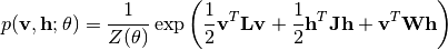
A Boltzmann machine (BM) is a generative probabilistic model that describes data through hidden layers. In particular, a deep belief network and a deep Boltzmann machine, which becomes increasingly popular in machine learning and its application domains, can be constructed by stacking multiple layers of BMs. In a generic Boltzmann machine, the joint distributions over both hidden units $\mathbf{h}$ and visible units $\mathbf{v}$ are given by

$p(\mathbf{v}, \mathbf{h}; \theta) = \frac{1}{Z(\theta)} \exp \left( \frac{1}{2} \mathbf{v}^T \mathbf{L} \mathbf{v} + \frac{1}{2} \mathbf{h}^T \mathbf{J} \mathbf{h} + \mathbf{v}^T \mathbf{W} \mathbf{h} \right)$

When $\mathbf{L}$ and $\mathbf{J}$ are zero matrices, this reduces to a restricted Boltzmann machine. By stakcing multiple layers of BMs, we obtain a deep Boltzmann machine as follows

$p(\mathbf{v}, \mathbf{h}; \theta) = \frac{1}{Z} \exp \left( \frac{1}{2} \mathbf{v}^T \mathbf{L} \mathbf{v} + \mathbf{v}^T \mathbf{W}_0 \mathbf{h}_1 + \sum_{l=1}^L \mathbf{h}_l^T \mathbf{J}_l \mathbf{h}_l + \sum_{l=1}^{L-1} \mathbf{h}_l^T \mathbf{W}_l \mathbf{h}_{l+1} \right)$

This probabilistic network, despite its complex internal structure, can be readily specified using the DSL as below

@model DeepBoltzmannMachine begin
    @hyperparam L::Int    # the number of latent layers
    @hyperparam nnodes::Vector{Int}   # the number of nodes in each layer
    @constant d::Int    # the dimension of observed sample
    @constant n::Int    # the number of observed samples

    # declare coefficient matrices
    @param L  :: Float64^(d, d)
    @param W0 :: Float64^(d, nnodes[1])

    for k = 1 : L
        @param J[k] :: Float64^(nnodes[k], nnodes[k])
    end

    for k = 1 : L-1
        @param W[k] :: Float64^(nnodes[k], nnodes[k+1])
    end

    # declare of variables
    for i = 1 : n
        obs[i] :: Float64^d
        for k = 1 : L
            latent[i][k] :: Float64^(nnodes[k])
        end
    end

    # samples
    for i = 1 : n
        let h = samples[i], v = obs[i]
            # intra-layer connections
            @expfac v' * L * v

            for k = 1 : L
                @expfac h[k]' * J[k] * h[k]
            end

            # inter-layer connections
            @expfac v' * W0 * h[1]

            for k = 1 : L-1
                @expfac h[k]' * W[k] * h[k+1]
            end
        end
    end
end

To learn this model from a set of samples, one can write

function learn_deepbm(x::Matrix{Float64}, nnodes::Vector{Int})
    # each column of x is a sample
    # nnodes specifies the number of nodes at each layer

    learn_model(DeepBoltzmannMachine(L = length(nnodes), nnodes=nnodes,
        d=size(x,1), n=size(x,2)), {:obs=>columns(x)})
end

mdl = learn_deepbm(x, [100, 50, 20])