Basics
OpenPPL is a domain-specific language built on top of Julia using macros. The language consists of two parts: model specification and query. In particular, a model specification formalizes a probabilistic model, which involves declaring variables and specifying relations between them; while a query specifies what is given and what is to be inferred.
Terminologies
Here is a list of terminologies that would be involved in the description.
- Variable
- A variable generally refers to an entity that can take a value of certain type. It can be a random variable directly associated with a distribution, a deterministic transformation of another variable, or just some value given by the user. The value of a variable can be given or unknown.
- Constant
- A value that is fixed when a query is constructed and fixed throughout the inference procedure. A constant is typically used to represent vector dimensions, model sizes, and hyper-parameters etc. Note that model parameters are typically considered as variables instead of constants. For example, a learning process can be formulated as a query that solves the parameter given a set of observations, where the parameter values can be iteratively updated.
- Domain
The domain of a variable refers to the set of possible values that it may take. Any Julia type (e.g.
Int,Float64) can be considered as a domain that contains any value of that type. This package also supports array domains and restrictive domains that contain only a subset of a specific type. Here are some examples:1 2 3 4 5
1..K            # integers between 1 and K
0.0..Inf        # all non-negative real values
Float64^n       # n-dimensional real vectors
Float64^(m,n)   # matrices of size (m, n)
(0.0..1.0)^m    # m-dimensional real vectors with all components in [0., 1.]
- Distribution
- From a programmatic standpoint, a distribution can be considered as a stochastic function that yields a random value in some domain. A distribution can accept zero or more arguments. A distribution should be stochastically pure, meaning that it always outputs the same value given the same arguments and the same state of the random number generator. Such purity makes it possible to reason about program structure and transform the model from one form to another.
- Factor
- A factor is a pure real-valued function. Here, “pure” means that it always output the same value given the same inputs. Factors are the core building blocks of a probabilistic model. A complex distribution is typically formulated as a set of variables connected by factors. Even a simple distribution (e.g. normal distribution) consists of a factor that connects between generated variables and parameters (which may be considered as a variable with fixed value).
Getting Started: Gaussian Mixture Model
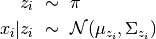
Here, we take the Gaussian Mixture Model as an example to illustrate how we can specify a probabilistic model using this Julia domain-specific language (DSL). A Gaussian Mixture Model is a generative model that combines several Gaussian components to approximate complex distributions (e.g. those with multiple modals.). A Gaussian mixture model is characterized by a prior distribution  and a set of Gaussian component parameters
  . The generative process is described as follows:
Model Specification
The model specification is given by
This model specification should be self-explanatory. However, it is still worth clarifying several aspects:
The macro
@modeldefines a model type namedGaussianMixtureModel, and creates an environment (delimited bybeginandend) for model formulation. All model types created by@modelis a sub type ofAbstractModel.The macro
@constantdeclaresd,K, andnas constants. The values of these constants need not be given in the specification. Instead, they are needed upon query. Particularly, to construct a model, one can writemdl = GaussianMixtureModel()
One can optionally fix the value of constants through keyword arguments in model construction, as below
mdl = GaussianMixtureModel(d = 2, K = 5)
Note: fixing constants upon model construction is generally unnecessary. However, it might be useful to fix them under certain circumstances to to simplify queries or restrict its use. Once a constant is fixed, it need not be specified again in the query.
The macro
@hyperparamdeclares hyper parameters. Hyper parameters are similar to constant technically, except that they typically refer to model configurations that may be changed during cross validation.Variables can be defined using the syntax as
variable-name :: domain. A for-loop can be used to declare multiple variables in the same domain. When the variable domain is clear from the context (e.g. the domain ofzandxcan be inferred from where they are drawn), the declaration can be omitted.The macro
@paramtags certain variables to be parameters. The information will be used in the learning algorithm to determine which variables are the parameters to estimate.The statement
variable-name ~ distributionintroduces a conditional distribution over variables, which will be translated into a factor during model compilation.
Generic Specification: Finite Mixture Model
The Gaussian mixture model can be considered as a special case in a generic family called Finite mixture model. Generally, the components of a finite mixture model can be arbitrary distributions. To capture the concept of generic distribution family, we introduce generic specification (or parametric specification), which can take type arguments.
The specification of the generic finite mixture model is given by
One may consider a generic specification above as a specification template. To obtain a Gaussian mixture model specification, we can use the @modelalias macro, as below:
The @modelalias macro allows introducing new constants and specializing the type parameters.
Queries
In machine learning, the most common queries that people would make include
- learning: estimate model parameters
- prediction: predict the value or marginal distribution over unknown variables, given a learned model and observed variables.
- evaluation: evaluate log-likelihood of observations with a given model
- sampling: draw a set of samples of certain variables
To simplify these common queries, we provide several functions.
Query
Query refers to the task of inferring the value or marginal distributions of unknown variables, given a set of known variables.
qlist is a list of variables or functions over variables that you want to infer. The function compile_query actually performs model compilation, analyzing model structure, choosing appropriate inference algorithms, and generating a closure q, which, when executed, actually performs the inference.
This query function here is very flexible. One can use it for prediction and sampling, etc.
Note that inputs to the function are symbols like :z or expressions like :(marginal(z)), which indicate what we want to query. It is incorrect to pass z or marginal(z) – the value of z or marginal(z) is unavailable before the inference.
Learning
Learning refers to the task of estimating model parameters given observed data. This can be considered as a special kind of query, which infers the values of model parameters, given observed data.
In the function learn_model, parameters(rmdl) returns a list of parameters as the query list. Then the statement q = compile_query(rmdl, parameters(rmdl), options) returns a query function q, such that q() executes the estimation procedure and returns the estimated model parameters. The following example shows how we can use this function to learn a Gaussian mixture model.
Here, learn_gmm is a light-weight wrapper of learn_model.
Evaluation
Evaluation refers to the task of evaluating log-pdf of samples with respect to a learned model.
# evaluate the logpdf of x with respect to a GMM
lp = query(rmdl, {:x=>columns(data)}, :(logpdf(x)))
Options
The compilation options that control how the query is compiled can be specified through the options argument in the query or learn_model function. The following is some examples
rmdl = learn_model(mdl, data, {:method=>"variational_em", :max_iter=>100, :tolerance=1.0e-6})
For sampling, we may use a different set of options
options = {
    :method=>"gibbs_sampling",  # choose to use Gibbs sampling
    :burnin=>5000,              # the number of burn-in iterations
    :lag=>100}                  # the interval between two samples to retain

samples = query(rmdl, {x:=>columns(data)}, :(samples(z, 100)), options)
Query Functions with Arguments
It is often desirable in practice that a query function can be applied to different data sets without being re-compiled. For this purpose, we introduce a function make_query_function. The following example illustrates its use:
Note that q is a closure that holds reference to the learned model, so you don’t have to pass the model as an argument into q. The following code use this mechanism to generate a sampler: