Nonparametric Models¶

Bayesian nonparametric models, such as DP mixture models, provide a flexible approach in which model structure (e.g. the number of components) can be adapted to data. The capability and effectiveness of such models have been proven in many applications.

This flexibility, however, leads to new questions to probabilistic programming – how to express models whose size/structure can vary. The Julia macro system makes it possible to address this problem in an elegant way due to is lazy evaluation nature.

Dirichlet Process Mixture Model¶

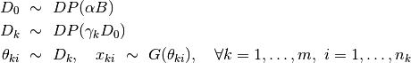
Dirichlet process mixture model (DPMM) is one of the most widely used in Bayesian nonparametrics. The formulation of DPMM is given by

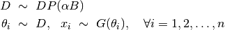
$D & \ \sim \ DP(\alpha B) \\ \theta_i & \ \sim \ D, \ \ x_i \ \sim \ G(\theta_i), \quad \forall i = 1, 2, \ldots, n$

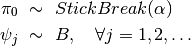
Here, $\alpha$ is the concentration paramater, $B$ is the base measure, and $G$ denotes the component models that generate the observed samples. The model specification for a DPMM is given as below. It has been shown that $D$ is almost surely discrete, and can be expressed in the followin form:

$D = \sum_{k=1}^\infty \pi_k \delta_{\phi_k}$

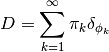
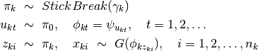
Hence, there exists positive probability that some of the components will be repeatedly sampled, and thus the number of distinct components is usually smaller than the number of samples. In practice, it is useful to construct a pool of components $\phi_1, \phi_2, \ldots$ , and introduce an indicator $z_i$ for each sample $x_i$ , such that $\theta_i = \phi_{z_i}$ . To make this explicit, we can reformulate the model as below

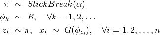
$\pi & \ \sim \ StickBreak(\alpha) \\ \phi_k & \ \sim \ B, \quad \forall k = 1, 2, \ldots \\ z_i & \ \sim \pi, \ \ x_i \ \sim \ G(\phi_{z_i}), \quad \forall i = 1, 2, \ldots, n$

Here, \pi, a sample from the stick breaking process, is an infinite sequence that sums to unity (i.e. $\sum_{i=1}^\infty \pi_i = 1$ ). The values of $pi$ are defined as

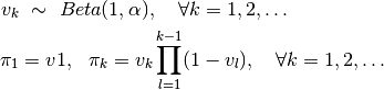
$v_k & \ \sim \ Beta(1, \alpha), \quad \forall k = 1, 2, \ldots \\ \pi_1 &= v1, \ \ \pi_k = v_k \prod_{l=1}^{k-1} (1 - v_l), \quad \forall k = 1, 2, \ldots$

The model specification for this formulation is given below

@model DPMixtureModel{B, G} begin
    @constant n::Int            # the number of observed samples
    @hyperparam alpha::Float64  # the concentration parameter

    pi ~ StickBreak(alpha)
    for k = 1 : Inf
        phi[k] ~ B
    end

    # samples
    for i = 1 : n
        z[i] ~ pi
        x[i] ~ G(phi[z[i]])
    end
end

Remarks:

The parametric setting makes it possible to use arbitrary base distribution $B$ and component $G$ here, with the same generic formulation.
In theory, $\pi$ is an infinite sequence, and therefore it is not feasible to completely instantiate a sample path of $\pi$ in computer. This variable may be marginalized out in the inference, and thus directly querying $\pi$ is not allowed.
$\phi$ has infinitely many components. However, only a finite number of them are needed in inference. The compiler should generate a lazy data structure that only memorizes the subset of components needed during the inference. In particular, phi[k] is constructed and memorized when there is an i such that k = z[i]. Some efforts (e.g. the LazySequences.jl) have demonstrated that lazy data structure can be implemented efficiently in Julia.

Hierarchical Dirichlet Processes¶

HDP is an extension of the DP mixture models, which allows groups of data to be modeled by different DPs that share components. The formulation of HDP is given below

$D_0 & \ \sim \ DP(\alpha B) \\ D_k & \ \sim \ DP(\gamma_k D_0) \\ \theta_{ki} & \ \sim \ D_k, \quad x_{ki} \ \sim \ G(\theta_{ki}), \quad \forall k = 1, \ldots, m, \ i = 1, \ldots, n_k$

Using $D_0$ as a base measure for the DP associated with each group, all groups share components in $D_0$ while allowing potentially infinite number of components. This formulation can be re-written (equivalently) using Pitman-Yor process, as follows

$\pi_0 & \ \sim \ StickBreak(\alpha) \\ \psi_j & \ \sim \ B, \quad \forall j = 1, 2, \ldots$

Then for each $k = 1, \ldots, m$ ,

$\pi_k & \ \sim \ StickBreak(\gamma_k) \\ u_{kt} & \ \sim \ \pi_0, \quad \phi_{kt} = \psi_{u_{kt}}, \quad t = 1, 2, \ldots \\ z_{ki} & \ \sim \ \pi_k, \quad x_{ki} \ \sim \ G(\phi_{k z_{ki}}), \quad i = 1, 2, \ldots, n_k$

Here is a brief description of this procedure:

To generate $D_0$ , we first draw an infinite multinomial distribution $\pi_0$ from a Pitman-Yor process with concentration parameter $\alpha$ , and draw each component $\psi_j$ from $B$ . Then $D_0 = \sum_{j=1}^\infty \pi_j \psi_j$ .
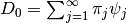Then for each group (say the k-th one), we draw $\pi_k$ from a stick breaking process and draw each component from $D_0$ . Note that drawing a component $\phi_{kt}$ from $D_0$ is equivalent to choosing one of the atoms in $D_0$ , which can be done in two steps: draw $u_{kt}$ from $\pi_0$ and then set $\phi_{kt} = \psi_{u_{kt}}$ . In other words, the $t$ -th component in the $k$ -th group is identical to the $u_{kt}$ -th component in $D_0$ .
Finally, to generate the $i$ -th sample in the $k$ -th group, denoted by $x_{ki}$ , we first draw $z_{ki}$ from $\pi_k$ and use the corresponding component $\phi_{kz_{ki}}$ to generate the sample.

This formulation can be expressed using the DSL as below:

@model HierarchicalDP{B, G} begin
    @constant m::Int           # the number of groups
    @constant ns::Vector{Int}  # the number of samples in each group
    @hyperparam alpha::Float64   # the base concentration
    @hyperparam gamma::Float64   # the group specific concentration

    # for D0
    pi0 ~ StickBreak(alpha)
    for j = 1 : Inf
        psi[j] ~ B
    end

    # each group
    for k = 1 : m
        pi[k] ~ StickBreak(gamma)

        # Dk
        for t = 1 : Inf
            u[k][t] ~ pi0
            phi[k][t] = psi[u[k][t]]
        end

        # samples
        for i = 1 : ns[k]
            z[k][t] ~ pi[k]
            x[k][i] ~ G(phi[z[k][t]])
        end
    end
end

Gaussian Processes¶

Gaussian process (GP) is another important stochastic process that is widely used in Bayesian modeling. Formally, a Gaussian process is defined to be a a function-valued distribution $X_t: t \in T$ , where $T$ can be arbitrary domain, such that any finite subset of values in $X_t$ is normally distributed. A Gaussian process is characterized by a mean function $\mu: T \rightarrow R$ and a positive definite covariance function 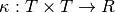$\kappa: T \times T \rightarrow R$ . The covariance function is typically given in a parametric form. The following is one that is widely used

$\kappa(s, t; \theta) = \theta_0 \delta_{s,t} + \theta_1 \exp ( -\theta_2 (s - t)^2 )$

In many application, the GP is considered to be hidden, and observations are a noisy transformation of the samples generated from the GP, as

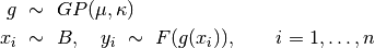
$g & \ \sim \ GP(\mu, \kappa) \\ x_i & \ \sim \ B, \quad y_i \ \sim \ F(g(x_i)), \quad \quad i = 1, \ldots, n$

The following model specification describes this model.

@model TransformedGaussProcess{B, F} begin
    @constant n::Int        # the number of observed samples

    # define mean and covariance function
    @param theta::Float^3
    mu(x) = 0.
    kappa(x, y) = theta[1] * delta(x, y) + theta[2] * exp(- theta[3] * abs2(x - y))

    # GP
    g ~ GaussianProcess(mu, kappa)

    # samples
    for i = 1 : n
        x[i] ~ B
        y[i] ~ F(g[x[i]])
    end
end

The GaussianProcess distribution here is a high-order stochastic function, which takes into two function arguments and generates another function. This is readily implementable in Julia, where functions are first-class citizens like in many functional programming languages.